Diferencia entre revisiones de «Hyperspectral Remote Sensing Scenes»
| (No se muestran 50 ediciones intermedias de 4 usuarios) | |||
| Línea 1: | Línea 1: | ||
Collected by: M Graña, MA Veganzons, B Ayerdi | |||
Here you can find information over some public available hyperspectral scenes. All of then are Earth Observation images taken from airbornes or satellites. | Here you can find information over some public available hyperspectral scenes. All of then are Earth Observation images taken from airbornes or satellites. | ||
You can find more information about hyperspectral sensors and remote sensing [http://www.ehu.es/ccwintco/index.php/Sensores-hiperespectrales here]. | |||
=== Indian Pines === | === Indian Pines === | ||
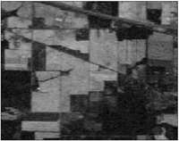
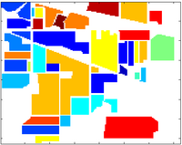
This scene was gathered by [http://aviris.jpl.nasa.gov/ AVIRIS sensor] over the Indian Pines test site in North-western Indiana and consists of 145\times145 pixels and 224 spectral reflectance bands in the wavelength range 0.4–2.5 10^(-6) meters. This scene is a subset of a larger one. The Indian Pines scene contains two-thirds agriculture, and one-third forest or other natural perennial vegetation. There are two major dual lane highways, a rail line, as well as some low density housing, other built structures, and smaller roads. Since the scene is taken in June some of the crops present, corn, soybeans, are in early stages of growth with less than 5% coverage. The ground truth available is designated into sixteen classes and is not all mutually exclusive. We have also reduced the number of bands to 200 by removing bands covering the region of water absorption: [104-108], [150-163], 220. Indian Pines data are available through [https://engineering.purdue.edu/~biehl/MultiSpec/hyperspectral.html Pursue's univeristy MultiSpec site]. | This scene was gathered by [http://aviris.jpl.nasa.gov/ AVIRIS sensor] over the Indian Pines test site in North-western Indiana and consists of 145\times145 pixels and 224 spectral reflectance bands in the wavelength range 0.4–2.5 10^(-6) meters. This scene is a subset of a larger one. The Indian Pines scene contains two-thirds agriculture, and one-third forest or other natural perennial vegetation. There are two major dual lane highways, a rail line, as well as some low density housing, other built structures, and smaller roads. Since the scene is taken in June some of the crops present, corn, soybeans, are in early stages of growth with less than 5% coverage. The ground truth available is designated into sixteen classes and is not all mutually exclusive. We have also reduced the number of bands to 200 by removing bands covering the region of water absorption: [104-108], [150-163], 220. Indian Pines data are available through [https://engineering.purdue.edu/~biehl/MultiSpec/hyperspectral.html Pursue's univeristy MultiSpec site]. | ||
* Download MATLAB data files: [[Media:indian_pines.mat|Indian Pines (6.0 MB)]] | [[Media:indian_pines_corrected.mat|corrected Indian Pines (5.7 MB)]] | [[Media:indian_pines_gt.mat|Indian Pines groundtruth (1.1 KB)]] | |||
[[Imagen:indian_pines_170.png|200px|thumb|Sample band of Indian Pines dataset]] | [[Imagen:indian_pines_170.png|200px|thumb|Sample band of Indian Pines dataset]] | ||
| Línea 82: | Línea 88: | ||
=== Salinas === | === Salinas === | ||
==== Salinas scene ==== | |||
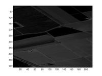
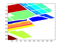
This scene was collected by the 224-band [http://aviris.jpl.nasa.gov/ AVIRIS sensor] over Salinas Valley, California, and is characterized by high spatial resolution (3.7-meter pixels). The area covered comprises 512 lines by 217 samples. As with Indian Pines scene, we discarded the 20 water absorption bands, in this case bands: [108-112], [154-167], 224. This image was available only as at-sensor radiance data. It includes vegetables, bare soils, and vineyard fields. Salinas groundtruth contains 16 classes. | This scene was collected by the 224-band [http://aviris.jpl.nasa.gov/ AVIRIS sensor] over Salinas Valley, California, and is characterized by high spatial resolution (3.7-meter pixels). The area covered comprises 512 lines by 217 samples. As with Indian Pines scene, we discarded the 20 water absorption bands, in this case bands: [108-112], [154-167], 224. This image was available only as at-sensor radiance data. It includes vegetables, bare soils, and vineyard fields. Salinas groundtruth contains 16 classes. | ||
* Download MATLAB data files: [[Media:salinas.mat|Salinas (26.3 MB)]] | [[Media:salinas_corrected.mat|corrected Salinas (25.3 MB)]] | [[Media:salinas_gt.mat|Salinas groundtruth (4.2 KB)]] | |||
[[Imagen:salinas_170.png|200px|thumb|Sample band of Salinas dataset]] | [[Imagen:salinas_170.png|200px|thumb|Sample band of Salinas dataset]] | ||
| Línea 163: | Línea 173: | ||
==== Salinas-A scene ==== | ==== Salinas-A scene ==== | ||
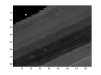
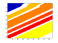
An small subscene of Salinas image, denoted Salinas-A, is usually used too. It comprises 86*83 pixels located within the same scene at [samples, lines] = [591-676, 158-240] and includes six classes. | An small subscene of Salinas image, denoted Salinas-A, is usually used too. It comprises 86*83 pixels located within the same scene at [samples, lines] = [591-676, 158-240] and includes six classes. | ||
* Download MATLAB data files: [[Media:salinasA.mat|Salinas-A (1.5 MB)]] | [[Media:salinasA_corrected.mat|corrected Salinas-A (1.5 MB)]] | [[Media:salinasA_gt.mat|Salinas-A groundtruth (587 Bytes)]] | |||
[[Imagen:salinasA_170.png|200px|thumb|Sample band of Salinas-A dataset]] | [[Imagen:salinasA_170.png|200px|thumb|Sample band of Salinas-A dataset]] | ||
| Línea 169: | Línea 181: | ||
{|style="border-collapse: collapse; border-width: 1px; border-style: solid; border-color: #000" align="center" style="text-align:center;" | {|style="border-collapse: collapse; border-width: 1px; border-style: solid; border-color: #000" align="center" style="text-align:center;" | ||
|- | |- | ||
!colspan="3"|Groundtruth classes for the Salinas-A and their respective samples number | !colspan="3"|Groundtruth classes for the Salinas-A scene and their respective samples number | ||
|- | |- | ||
!style="border-style: solid; border-width: 1px"| # | !style="border-style: solid; border-width: 1px"| # | ||
| Línea 204: | Línea 216: | ||
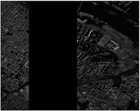
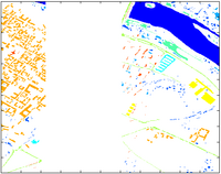
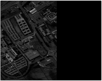
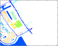
These are two scenes acquired by the [http://www.opairs.aero/rosis_en.html ROSIS sensor] during a flight campaign over Pavia, nothern Italy. The number of spectral bands is 102 for Pavia Centre and 103 for Pavia University. Pavia Centre is a 1096*1096 pixels image, and Pavia University is 610*610 pixels, but some of the samples in both images contain no information and have to be discarded before the analysis. The geometric resolution is 1.3 meters. Both image groundtruths differenciate 9 classes each. It can be seen the discarded samples in the figures as abroad black strips. | These are two scenes acquired by the [http://www.opairs.aero/rosis_en.html ROSIS sensor] during a flight campaign over Pavia, nothern Italy. The number of spectral bands is 102 for Pavia Centre and 103 for Pavia University. Pavia Centre is a 1096*1096 pixels image, and Pavia University is 610*610 pixels, but some of the samples in both images contain no information and have to be discarded before the analysis. The geometric resolution is 1.3 meters. Both image groundtruths differenciate 9 classes each. It can be seen the discarded samples in the figures as abroad black strips. | ||
Pavia scenes were provided by [http://tlclab.unipv.it/sito_tlc/people.do?id=pgamba Prof. | Pavia scenes were provided by [http://tlclab.unipv.it/sito_tlc/people.do?id=pgamba Prof. Paolo Gamba] from the [http://tlclab.unipv.it Telecommunications and Remote Sensing Laboratory], [http://www.unipv.eu Pavia university] (Italy). | ||
==== Pavia Centre scene ==== | ==== Pavia Centre scene ==== | ||
* Download MATLAB data files: [[Media:pavia.mat|Pavia Centre (123.6 MB)]] | [[Media:pavia_gt.mat|Pavia Centre groundtruth (34.1 KB)]] | |||
[[Imagen:pavia_60.png|200px|thumb|Sample band of Pavia Centre dataset]] | [[Imagen:pavia_60.png|200px|thumb|Sample band of Pavia Centre dataset]] | ||
| Línea 257: | Línea 271: | ||
==== Pavia University scene ==== | ==== Pavia University scene ==== | ||
* Download MATLAB data files: [[Media:paviaU.mat|Pavia University (33.2 MB)]] | [[Media:paviaU_gt.mat|Pavia University groundtruth (10.7 KB)]] | |||
[[Imagen:paviaU_60.png|200px|thumb|Sample band of Pavia University dataset]] | [[Imagen:paviaU_60.png|200px|thumb|Sample band of Pavia University dataset]] | ||
| Línea 270: | Línea 286: | ||
|- | |- | ||
|style="border-style: solid; border-width: 1px"| 1 | |style="border-style: solid; border-width: 1px"| 1 | ||
|style="border-style: solid; border-width: 1px"| | |style="border-style: solid; border-width: 1px"| Asphalt | ||
|style="border-style: solid; border-width: 1px"| | |style="border-style: solid; border-width: 1px"| 6631 | ||
|- | |- | ||
|style="border-style: solid; border-width: 1px"| 2 | |style="border-style: solid; border-width: 1px"| 2 | ||
|style="border-style: solid; border-width: 1px"| | |style="border-style: solid; border-width: 1px"| Meadows | ||
|style="border-style: solid; border-width: 1px"| | |style="border-style: solid; border-width: 1px"| 18649 | ||
|- | |- | ||
|style="border-style: solid; border-width: 1px"| 3 | |style="border-style: solid; border-width: 1px"| 3 | ||
|style="border-style: solid; border-width: 1px"| | |style="border-style: solid; border-width: 1px"| Gravel | ||
|style="border-style: solid; border-width: 1px"| | |style="border-style: solid; border-width: 1px"| 2099 | ||
|- | |- | ||
|style="border-style: solid; border-width: 1px"| 4 | |style="border-style: solid; border-width: 1px"| 4 | ||
|style="border-style: solid; border-width: 1px"| | |style="border-style: solid; border-width: 1px"| Trees | ||
|style="border-style: solid; border-width: 1px"| | |style="border-style: solid; border-width: 1px"| 3064 | ||
|- | |- | ||
|style="border-style: solid; border-width: 1px"| 5 | |style="border-style: solid; border-width: 1px"| 5 | ||
|style="border-style: solid; border-width: 1px"| Painted metal sheets | |style="border-style: solid; border-width: 1px"| Painted metal sheets | ||
|style="border-style: solid; border-width: 1px"| | |style="border-style: solid; border-width: 1px"| 1345 | ||
|- | |- | ||
|style="border-style: solid; border-width: 1px"| 6 | |style="border-style: solid; border-width: 1px"| 6 | ||
|style="border-style: solid; border-width: 1px"| | |style="border-style: solid; border-width: 1px"| Bare Soil | ||
|style="border-style: solid; border-width: 1px"| | |style="border-style: solid; border-width: 1px"| 5029 | ||
|- | |- | ||
|style="border-style: solid; border-width: 1px"| 7 | |style="border-style: solid; border-width: 1px"| 7 | ||
|style="border-style: solid; border-width: 1px"| | |style="border-style: solid; border-width: 1px"| Bitumen | ||
|style="border-style: solid; border-width: 1px"| | |style="border-style: solid; border-width: 1px"| 1330 | ||
|- | |- | ||
|style="border-style: solid; border-width: 1px"| 8 | |style="border-style: solid; border-width: 1px"| 8 | ||
|style="border-style: solid; border-width: 1px"| | |style="border-style: solid; border-width: 1px"| Self-Blocking Bricks | ||
|style="border-style: solid; border-width: 1px"| | |style="border-style: solid; border-width: 1px"| 3682 | ||
|- | |- | ||
|style="border-style: solid; border-width: 1px"| 9 | |style="border-style: solid; border-width: 1px"| 9 | ||
|style="border-style: solid; border-width: 1px"| | |style="border-style: solid; border-width: 1px"| Shadows | ||
|style="border-style: solid; border-width: 1px"| | |style="border-style: solid; border-width: 1px"| 947 | ||
|} | |} | ||
=== Cuprite === | |||
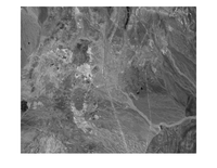
This data sets can be retrieved from [http://aviris.jpl.nasa.gov/ AVIRIS NASA] site. Among the many datasets available, the .mat archive posted here corresponds to the ''f970619t01p02_r02_sc03.a.rfl'' reflectance file. | |||
* Download MATLAB data file: [[Media:cuprite_f970619t01p02_r02_sc03.a.rfl.mat|Cuprite (95.3 MB)]] | |||
[[Imagen:cuprite_false_greyscale.png|200px|thumb|False greyscale image of Cuprite sample.]] | |||
=== Kennedy Space Center (KSC) === | |||
The NASA AVIRIS (Airborne Visible/Infrared Imaging Spectrometer) instrument acquired data over the Kennedy Space Center (KSC), Florida, on March 23, 1996. AVIRIS acquires data in 224 bands of 10 nm width with center wavelengths from 400 - 2500 nm. The KSC data, acquired from an altitude of approximately 20 km, have a spatial resolution of 18 m. After removing water absorption and low SNR bands, 176 bands were used for the analysis. Training data were selected using land cover maps derived from color infrared photography provided by the Kennedy Space Center and Landsat Thematic Mapper (TM) imagery. The vegetation classification scheme was developed by KSC personnel in an effort to define functional types that are discernable at the spatial resolution of Landsat and these AVIRIS data. Discrimination of land cover for this environment is difficult due to the similarity of spectral signatures for certain vegetation types. For classification purposes, 13 classes representing the various land cover types that occur in this environment were defined for the site. | |||
* Take a fast look to the data! [http://www.ehu.es/ccwintco/uploads/2/28/KSC.gif] | |||
* Download MATLAB data file: [http://www.ehu.es/ccwintco/uploads/2/26/KSC.mat Kennedy Space Center (KSC) (56.8 MB)] | |||
* Download MATLAB ground truth file: [http://www.ehu.es/ccwintco/uploads/a/a6/KSC_gt.mat KSC gt (3.2 kB)] | |||
* [[Corrected version offered by Ilya Kavalerov]] | |||
=== Botswana === | |||
The NASA EO-1 satellite acquired a sequence of data over the Okavango Delta, Botswana in 2001-2004. The Hyperion sensor on EO-1 acquires data at 30 m pixel resolution over a 7.7 km strip in 242 bands covering the 400-2500 nm portion of the spectrum in 10 nm windows. Preprocessing of the data was performed by the UT Center for Space Research to mitigate the effects of bad detectors, inter-detector miscalibration, and intermittent anomalies. Uncalibrated and noisy bands that cover water absorption features were removed, and the remaining 145 bands were included as candidate features: [10-55, 82-97, 102-119, 134-164, 187-220]. The data analyzed in this study, acquired May 31, 2001, consist of observations from 14 identified classes representing the land cover types in seasonal swamps, occasional swamps, and drier woodlands located in the distal portion of the Delta. | |||
* Take a fast look to the data! [http://www.ehu.es/ccwintco/uploads/0/05/Botswana.gif] | |||
* Download MATLAB data file: [http://www.ehu.es/ccwintco/uploads/7/72/Botswana.mat Botswana (78.9 MB)] | |||
* Download MATLAB ground truth file: [http://www.ehu.es/ccwintco/uploads/5/58/Botswana_gt.mat Botswana gt (4.0 kB)] | |||
===anomaly detection === | |||
[http://xudongkang.weebly.com/data-sets.html Xudong Kang dataset for anomaly detection] | |||
Revisión actual - 19:27 12 jul 2021
Collected by: M Graña, MA Veganzons, B Ayerdi
Here you can find information over some public available hyperspectral scenes. All of then are Earth Observation images taken from airbornes or satellites.
You can find more information about hyperspectral sensors and remote sensing here.
Indian Pines
This scene was gathered by AVIRIS sensor over the Indian Pines test site in North-western Indiana and consists of 145\times145 pixels and 224 spectral reflectance bands in the wavelength range 0.4–2.5 10^(-6) meters. This scene is a subset of a larger one. The Indian Pines scene contains two-thirds agriculture, and one-third forest or other natural perennial vegetation. There are two major dual lane highways, a rail line, as well as some low density housing, other built structures, and smaller roads. Since the scene is taken in June some of the crops present, corn, soybeans, are in early stages of growth with less than 5% coverage. The ground truth available is designated into sixteen classes and is not all mutually exclusive. We have also reduced the number of bands to 200 by removing bands covering the region of water absorption: [104-108], [150-163], 220. Indian Pines data are available through Pursue's univeristy MultiSpec site.
- Download MATLAB data files: Indian Pines (6.0 MB) | corrected Indian Pines (5.7 MB) | Indian Pines groundtruth (1.1 KB)
| Groundtruth classes for the Indian Pines scene and their respective samples number | ||
|---|---|---|
| # | Class | Samples |
| 1 | Alfalfa | 46 |
| 2 | Corn-notill | 1428 |
| 3 | Corn-mintill | 830 |
| 4 | Corn | 237 |
| 5 | Grass-pasture | 483 |
| 6 | Grass-trees | 730 |
| 7 | Grass-pasture-mowed | 28 |
| 8 | Hay-windrowed | 478 |
| 9 | Oats | 20 |
| 10 | Soybean-notill | 972 |
| 11 | Soybean-mintill | 2455 |
| 12 | Soybean-clean | 593 |
| 13 | Wheat | 205 |
| 14 | Woods | 1265 |
| 15 | Buildings-Grass-Trees-Drives | 386 |
| 16 | Stone-Steel-Towers | 93 |
Salinas
Salinas scene
This scene was collected by the 224-band AVIRIS sensor over Salinas Valley, California, and is characterized by high spatial resolution (3.7-meter pixels). The area covered comprises 512 lines by 217 samples. As with Indian Pines scene, we discarded the 20 water absorption bands, in this case bands: [108-112], [154-167], 224. This image was available only as at-sensor radiance data. It includes vegetables, bare soils, and vineyard fields. Salinas groundtruth contains 16 classes.
- Download MATLAB data files: Salinas (26.3 MB) | corrected Salinas (25.3 MB) | Salinas groundtruth (4.2 KB)
| Groundtruth classes for the Salinas scene and their respective samples number | ||
|---|---|---|
| # | Class | Samples |
| 1 | Brocoli_green_weeds_1 | 2009 |
| 2 | Brocoli_green_weeds_2 | 3726 |
| 3 | Fallow | 1976 |
| 4 | Fallow_rough_plow | 1394 |
| 5 | Fallow_smooth | 2678 |
| 6 | Stubble | 3959 |
| 7 | Celery | 3579 |
| 8 | Grapes_untrained | 11271 |
| 9 | Soil_vinyard_develop | 6203 |
| 10 | Corn_senesced_green_weeds | 3278 |
| 11 | Lettuce_romaine_4wk | 1068 |
| 12 | Lettuce_romaine_5wk | 1927 |
| 13 | Lettuce_romaine_6wk | 916 |
| 14 | Lettuce_romaine_7wk | 1070 |
| 15 | Vinyard_untrained | 7268 |
| 16 | Vinyard_vertical_trellis | 1807 |
Salinas-A scene
An small subscene of Salinas image, denoted Salinas-A, is usually used too. It comprises 86*83 pixels located within the same scene at [samples, lines] = [591-676, 158-240] and includes six classes.
- Download MATLAB data files: Salinas-A (1.5 MB) | corrected Salinas-A (1.5 MB) | Salinas-A groundtruth (587 Bytes)
| Groundtruth classes for the Salinas-A scene and their respective samples number | ||
|---|---|---|
| # | Class | Samples |
| 1 | Brocoli_green_weeds_1 | 391 |
| 2 | Corn_senesced_green_weeds | 1343 |
| 3 | Lettuce_romaine_4wk | 616 |
| 4 | Lettuce_romaine_5wk | 1525 |
| 5 | Lettuce_romaine_6wk | 674 |
| 6 | Lettuce_romaine_7wk | 799 |
Pavia Centre and University
These are two scenes acquired by the ROSIS sensor during a flight campaign over Pavia, nothern Italy. The number of spectral bands is 102 for Pavia Centre and 103 for Pavia University. Pavia Centre is a 1096*1096 pixels image, and Pavia University is 610*610 pixels, but some of the samples in both images contain no information and have to be discarded before the analysis. The geometric resolution is 1.3 meters. Both image groundtruths differenciate 9 classes each. It can be seen the discarded samples in the figures as abroad black strips.
Pavia scenes were provided by Prof. Paolo Gamba from the Telecommunications and Remote Sensing Laboratory, Pavia university (Italy).
Pavia Centre scene
- Download MATLAB data files: Pavia Centre (123.6 MB) | Pavia Centre groundtruth (34.1 KB)
| Groundtruth classes for the Pavia centre scene and their respective samples number | ||
|---|---|---|
| # | Class | Samples |
| 1 | Water | 824 |
| 2 | Trees | 820 |
| 3 | Asphalt | 816 |
| 4 | Self-Blocking Bricks | 808 |
| 5 | Bitumen | 808 |
| 6 | Tiles | 1260 |
| 7 | Shadows | 476 |
| 8 | Meadows | 824 |
| 9 | Bare Soil | 820 |
Pavia University scene
- Download MATLAB data files: Pavia University (33.2 MB) | Pavia University groundtruth (10.7 KB)
| Groundtruth classes for the Pavia University scene and their respective samples number | ||
|---|---|---|
| # | Class | Samples |
| 1 | Asphalt | 6631 |
| 2 | Meadows | 18649 |
| 3 | Gravel | 2099 |
| 4 | Trees | 3064 |
| 5 | Painted metal sheets | 1345 |
| 6 | Bare Soil | 5029 |
| 7 | Bitumen | 1330 |
| 8 | Self-Blocking Bricks | 3682 |
| 9 | Shadows | 947 |
Cuprite
This data sets can be retrieved from AVIRIS NASA site. Among the many datasets available, the .mat archive posted here corresponds to the f970619t01p02_r02_sc03.a.rfl reflectance file.
- Download MATLAB data file: Cuprite (95.3 MB)
Kennedy Space Center (KSC)
The NASA AVIRIS (Airborne Visible/Infrared Imaging Spectrometer) instrument acquired data over the Kennedy Space Center (KSC), Florida, on March 23, 1996. AVIRIS acquires data in 224 bands of 10 nm width with center wavelengths from 400 - 2500 nm. The KSC data, acquired from an altitude of approximately 20 km, have a spatial resolution of 18 m. After removing water absorption and low SNR bands, 176 bands were used for the analysis. Training data were selected using land cover maps derived from color infrared photography provided by the Kennedy Space Center and Landsat Thematic Mapper (TM) imagery. The vegetation classification scheme was developed by KSC personnel in an effort to define functional types that are discernable at the spatial resolution of Landsat and these AVIRIS data. Discrimination of land cover for this environment is difficult due to the similarity of spectral signatures for certain vegetation types. For classification purposes, 13 classes representing the various land cover types that occur in this environment were defined for the site.
- Take a fast look to the data! [1]
- Download MATLAB data file: Kennedy Space Center (KSC) (56.8 MB)
- Download MATLAB ground truth file: KSC gt (3.2 kB)
* Corrected version offered by Ilya Kavalerov
Botswana
The NASA EO-1 satellite acquired a sequence of data over the Okavango Delta, Botswana in 2001-2004. The Hyperion sensor on EO-1 acquires data at 30 m pixel resolution over a 7.7 km strip in 242 bands covering the 400-2500 nm portion of the spectrum in 10 nm windows. Preprocessing of the data was performed by the UT Center for Space Research to mitigate the effects of bad detectors, inter-detector miscalibration, and intermittent anomalies. Uncalibrated and noisy bands that cover water absorption features were removed, and the remaining 145 bands were included as candidate features: [10-55, 82-97, 102-119, 134-164, 187-220]. The data analyzed in this study, acquired May 31, 2001, consist of observations from 14 identified classes representing the land cover types in seasonal swamps, occasional swamps, and drier woodlands located in the distal portion of the Delta.
- Take a fast look to the data! [2]
- Download MATLAB data file: Botswana (78.9 MB)
- Download MATLAB ground truth file: Botswana gt (4.0 kB)
